When Molecules Spin: A Story of Bulk Viscosity

Introduction

Look closely enough at the air in this room and it stops being a smooth substance. It becomes a crowd of molecules, and most of them are not simple specks. They are pairs of atoms joined together, tumbling end over end as they fly.

That tumbling matters more than it sounds. Squeeze a gas and it pushes back, but not all of it and not all at once. Part of the effort you spend goes into setting molecules spinning faster, and that share comes back as pressure only later, once the molecules have collided with one another many times over. The gas answers on a delay.

Engineers have a name for that delay: bulk viscosity. You will never notice it inflating a bicycle tire. It becomes hard to ignore wherever a gas is pushed hard and fast, such as the searing shock layer ahead of a returning spacecraft, or the thin streams of gas that machines move through near-vacuum. Predicting those flows means getting the spin right.

Most of the mathematics of rarefied gases, though, was worked out for the simplest imaginable case, in which a molecule carries energy only as motion through space. Real gases carry it as spin as well, and any model hoping to describe them has to say what becomes of that spin each time two molecules meet.

The Hidden Reservoir

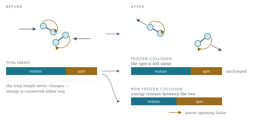
Consider two nitrogen molecules approaching each other. Each carries two kinds of energy: the energy of flying through space, and the energy of spinning about its own axis. When they collide, the total is conserved, but how it is divided is not fixed.

Sometimes the collision is effectively elastic: the molecules deflect, exchange some speed, and go on spinning as before. The internal reservoir is untouched. Other times the collision reaches into that reservoir, and a molecule leaves spinning faster than it arrived, having paid for it out of its translational motion, or the reverse.

A Dial Between Two Idealized Collisions

Writing down a collision model that captures this is harder than it looks, because a real collision is neither purely one nor the other. The model we build on, due to Djordjić, Oblapenko, Pavić-Čolić and Torrilhon, takes a pragmatic route: describe the two extremes exactly, then mix them.

The two extremes are the frozen collision, which is elastic and leaves every molecule's internal energy exactly as it found it, and the non-frozen collision, which redistributes energy freely between motion and spin according to a well-established statistical recipe. The real gas is modeled as a convex combination of the two. A single number, call it $\omega$, sets the mix:

$\text{collisions} \;=\; \omega \times (\text{non-frozen}) \;+\; (1-\omega) \times (\text{frozen})$

If $\omega$ is one, every collision shuffles energy between motion and spin. If $\omega$ is zero, none of them do and the internal energy is inert cargo. Anything in between is a statement about how often a molecular encounter actually manages to change a molecule's rotation. A second parameter refines this further, letting the likelihood of exchange depend on how much internal energy the molecules already carry, since a molecule already spinning fast behaves differently from one barely turning.

Two numbers, then, stand between an abstract collision model and a real gas. The question is whether they are enough.

Three Gases, Two Parameters

Two measurable quantities test a collision model where it matters. The Prandtl number compares how readily a gas transports momentum against how readily it conducts heat. The bulk-to-shear viscosity ratio measures the delayed response to compression, the effect that exists only because molecules can spin. Both have been measured for common gases to good precision.

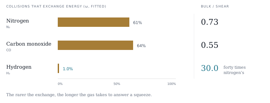
We fitted the two model parameters inside our own collision operator, for nitrogen, carbon monoxide and hydrogen, and asked it to reproduce both measurements at once. It does so for all three gases, with parameters that stay inside the range where the model remains physically admissible.

Gas	Exchange fraction $\omega$	Prandtl	Bulk / shear
Nitrogen	0.607	0.717	0.73
Carbon monoxide	0.638	0.743	0.55
Hydrogen	0.010	0.686	30.0

The Prandtl numbers and viscosity ratios are the measured values, reproduced by the fitted operator.

Why Hydrogen Is the Outlier

Hydrogen's row stands apart. One collision in a hundred does anything at all to the molecules' rotation, and its bulk viscosity is thirty times its shear viscosity, unusually large for a common gas.

The two facts are connected. Hydrogen is the lightest molecule there is, and its two atoms sit very close together, which makes it hard to set spinning: its rotational states are spaced far apart in energy, so a typical collision at room temperature does not carry enough of the right kind of energy to nudge it from one to the next. The rotation is effectively locked. And a gas whose internal reservoir fills only once every hundred collisions takes a long time to come back into balance after it is compressed, which is precisely what a large bulk viscosity means.

It is worth noting what the model did here. We did not tell it that hydrogen is a slow relaxer. We gave it two measured transport coefficients and let it find the mix that reproduces them, and it recovered a picture of hydrogen's molecular behavior that matches what spectroscopy independently tells us. The fitted parameter turns out to mean something.

Making It Fast Enough to Use

None of this would be useful if evaluating the model were too slow. Once the molecules can spin, the collision operator becomes a twelve-dimensional integral, and the naive way of storing and applying it becomes impractical well before the resolutions engineering actually needs.

The way through is a piece of mathematics from quantum angular momentum theory, the Wigner–Eckart theorem, which splits the operator into a sparse geometric part that knows about rotations in space and a dense physical part that knows about the collision itself. The geometry is universal; only the small dense part depends on the gas. In our implementation for spinning molecules that factorization compresses storage by roughly three orders of magnitude at practical resolutions and makes the contraction substantially faster. We wrote about how that works, and how it maps onto modern accelerators, in an earlier post.

What it buys us here is room to treat the physics carefully. Fitting a collision model to measured transport data means evaluating the operator many times over, at resolutions high enough that the answer is the model's and not the numerical method's. That is only possible if each evaluation is cheap.

Closing

A gas model earns its place by predicting something it was not tuned for. The next step is exactly that: taking these calibrated operators into flows such as nozzle expansions, shock layers and low-pressure chambers, where the gas is far from equilibrium and no single temperature describes it, and comparing against measurements that played no part in the fit.

The machinery is now in place. At Simkinetic, we are building the deterministic solvers that put it to work on the gases engineers actually use.